Stroop, flanker, and go-nogo tasks in OpenSesame

Stroop, flanker, and go-nogo tasks in OpenSesame¶

Note: The text below is adapted from the OpenSesame guide by James E. Bartlett licensed under CC-By Attribution 4.0 International.

Tutorial 1. Stroop Task¶

Creating the Stroop task¶

To get a look at OpenSesame, we will first create one of the simplest and most famous psychology experiments, the Stroop task. This demonstrates the automaticity of reading as identifying the font colour of a congruent word (e.g. blue) is faster than identifying the font colour of an incongruent word (e.g. blue). When the word and colour are incongruent, the interference causes a delay in identifying the colour of the font. We will create a single block of trials to demonstrate the task. As you go through the guide, I recommend saving your experiment every time you reach a new sub-heading like the next line.

Creating a new experiment¶

If you open OpenSesame on your computer, you should get a window that looks like this:

To help you start an experiment, there are some templates that you can use. We are going to use the default template as we are going to make a single block of trials from scratch to demonstrate the building blocks of OpenSesame. Once you click on this, a new screen will appear and you will be able to change any of the general properties of the task. It is a good idea to give your experiment an informative name. You can do this by clicking where it says New experiment in blue, and editing the text. Press the return key to save the new name. Make sure you change the resolution to your monitor’s dimensions. If you are not sure what the resolution of your monitor is, you can look in the display settings of your computer. Once you have changed these, the general properties window should look like this:

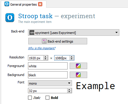
There are a few settings to explain here. Foreground and background refers to the colour of the screen and the elements displayed on it. We will keep the background black so the participant does not have to look at a dazzling white screen, and the foreground white to make it easy to read on a black background. I would also recommend increasing the default size of the font to 32, as 18 is too small to read and it saves you changing it every time you create a new component.

The building blocks of creating an experiment¶

Before making the Stroop task, we will go over some of the basics of structuring an experiment in OpenSesame. The design of your experiment will be shown in the Overview window, and it is displayed sequentially down the screen from the components at the start of the experiment to the components at the end of the experiment. The backbone of an experiment is created through loop and sequence components. A loop component repeats what is inside it and defines any variables to use. A sequence component contains other components such as a screen showing text that make up a single trial. Therefore, you would place a sequence component within a loop component to control how many times the sequence is repeated. Drag a loop component and place it after welcome in the overview window, and drag a sequence component and place it inside the loop. When you release the sequence, it will ask whether you want it placing into the loop or after the loop. Press into the loop and make sure they are both given informative names such as block_loop for the loop component and trial_sequence for the sequence component. For the names of components, there are a number of rules you need to follow. They cannot start with numbers, and you cannot include any spaces. If you need spaces to make it easier to read, use an underscore. You should now have a window that looks like this: Therefore, once we define our variables later, trial_sequence and everything in it will repeat for however many times you specify in block_loop. We will now create a single trial within trial_sequence. In most psychology experiments, you include a fixation cross to start a trial and focus the participant’s attention in the location where you will be presenting the stimulus.

Creating the fixation dot¶

This can be created using a sketchpad component . This is a very flexible component where you can present text, shapes, and images. The sketchpad window has a list of elements on the left hand side and a black screen with green lines to show where on the screen the elements would be placed. OpenSesame has a very handy fixation cross element called fixdot . Click on the fixdot element and this will turn your mouse into a pen icon. If you move the mouse around the black gridded screen, the coordinates are shown in the top right corner, and will change as you move around the screen. Place the fixdot element at 0,0 in the middle of the screen where the two green lines meet. This will place the fixdot in that position. There are two more things to change. Firstly, we can modify how long the stimuli are presented for by changing Duration. The default is keypress which would mean the screen will not disappear until the participant presses a button. We can change this to 500 to make the screen disappear after 500ms. Whenever you specify a duration in OpenSesame, it is stated in milliseconds. Therefore, to present something for 1 second, we would need to write 1000. Finally, we can change the name of the component to something informative such as fixation. You should now have a screen that looks like this:

Creating the word component¶

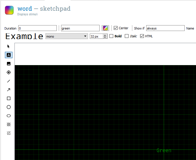
In the Stroop task, participants are shown colour words and the font is either the same colour as the word (congruent) or a different colour to the word (incongruent). Therefore, the next thing we need to do is create another sketchpad component to present the words. Drag a sketchpad component and place it after fixation in the trial sequence. Name it word to keep track of all the components. This time instead of inserting a fixation cross, we need a text element . After you have selected the text element, change the colour to green (all lowercase, it will say white by default). This will turn your mouse into a pen, and you need to click in the middle of the screen at 0,0 again to place it. When you click, it will ask you to enter some text. For now, just enter ‘Green’ as we want to show the participants colour words. This time, change Duration to 0. This does not mean that we never want it appearing on the screen, but we want it to only remain on the screen until a participant makes a response, which will require the next component keyboard_response. For the word component, you should have a window that looks like this:

Creating the keyboard response component¶

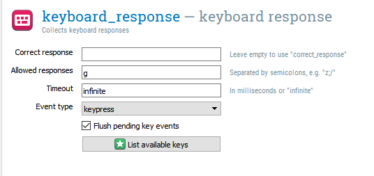
The next component is keyboard_response . Drag this from the menu and place it after word. We need this to tell OpenSesame which keyboard responses are allowed and which responses are correct. For now, we only have one green word, so the only response we need is ‘g’. If you are ever unsure of what the valid name of the key you need is, click on List available keys. We will not specify a correct response yet. We can leave Timeout to infinite, so the word will remain on the screen until the participant presses ‘g’ on the keyboard. As we set the duration of the word component to 0, the amount of time it is presented for is determined by keyboard_response. A keyboard response component does not display on the screen, so it keeps the display from the previous sketchpad component. A common mistake is to set a time for both components. This would not allow you to record any response until the Duration of the word component has ended. This could really confuse participants as they would have to respond twice for the trial to end. You should now have a screen that looks like this for keyboard_response:

Creating a blank screen¶

After the keyboard response, we will place another sketchpad component to signal the end of the trial. This time it will just be a blank screen presented for 200ms. You can do this yourself based on the previous sketchpad components and name it blank. We do not need to add any text or fixdot elements.

Creating the logger component¶

The next component that we need is a logger to save the data. OpenSesame does not save the responses by default, so you need to create a logger to save the data from each trial. Drag a logger component and place it after blank. For most experiments, you can just keep the default option here. It just saves every available variable on each trial.

Creating the end of experiment screen¶

The final component we need is a screen to tell the participant the experiment has finished. Without this, the experiment just closes which can make the participant panic and think they have done something wrong. Create a new sketchpad component called end_experiment and place it after block_loop. Make sure it is not in trial_sequence. If you drop it on block_loop, you can select insert after block_loop. Here we just need a brief message saying ‘The experiment has now finished. Press any key to exit’. In order to create this, select a text element , click in the middle of the screen, and enter the message. Now the participant is fully aware that the experiment has finished successfully. Make sure Duration is set to keypress. You should now have an experiment that looks like this in the Overview window:

Modifying the welcome message¶

The final thing to do before we test whether the experiment works is to change welcome. By default, this lists the version of OpenSesame that you are using. You can edit the pre-existing text by hovering over the text until it turns a light grey colour, and double-clicking. Change the text to something like ‘Welcome to the experiment, press any key to begin.’. We will make this more informative later on, but for now, this will do. All that matters is this sketchpad component has a keypress duration, as we want the participant to start the experiment when they are ready.

Time to test the experiment¶

Now it is time to make sure everything works! In the menu, there are three arrow buttons. If you were collecting data from a participant, you would press the big green triangle to run the experiment full screen. The two green triangles runs the experiment in a separate window. The two blue triangles allow you to quickly run the experiment in a separate screen to make sure everything is working. It is usually a good idea to test your experiment using quick run, as if your experiment crashes, you can force it to quit. If you click quick run, your experiment should successfully run in a small window. If it does not run, look back at all of the instructions and make sure you have not made any typos, and all the components are where they should be. Remember to press ‘g’ to indicate the color is green. We only have one trial up to yet, so it will only last around one second. However, it is helpful to keep testing an experiment to make sure it works before you add something else. It makes it much easier to debug your experiment if you know it worked previously. This means you only need to investigate the changes you have made since it last worked. Your sanity will thank you if you make incremental changes, saving and running the experiment after every addition. Now that we know one trial works, we can add in multiple words and make the colour of the word change.

Manipulating the presentation of word and colour¶

When we created the word component, we specified green as the word and colour. For the Stroop task, we want different words and colours depending on the condition. Therefore, we need to make both the word and colour variable for each trial. We need to do this in two steps. Firstly, we need to specify our conditions in block_loop (remember this is where we define our variables and control how many times sequence runs). We then need to change word to allow the word and colour to change every trial. We will start with block_loop.

Editing the block_loop component¶

If you click on block_loop, it looks like an Excel sheet with lots of cells. This is where we can define our variables and conditions. The rules here are every column is a variable, and each row is an individual condition. The variables must have unique names, so you cannot repeat a variable name in the same or a different loop component. The first column will be called ‘empty_column’ by default. We will change this to ‘word’. We will change the second column to ‘colour’. It makes it easier if you use lower case letters as the variable names are case sensitive. We then need to populate the cells. We will have four words and colours: red, blue, yellow, and green. We want there to be some congruent and incongruent trials, so write each colour twice in the word column. In the colour column, we will pair red with blue, and yellow with green. So for each word, you should have one congruent colour and one incongruent colour. The grid should look like this:

We also need some additional variables that will be helpful for analysing the data later. We need a column called ‘congruent’ and a column called ‘correct_resp’. In the congruent column, write a 1 for every time the word and colour match, and a 0 for every time they do not match. In programming, 1 usually means true and 0 usually means false. This means that when we get the data afterwards, we can sort the responses by congruency and calculate whether the reaction times are longer in the incongruent condition. We also need to specify what is the correct response in order to use it in keyboard_response. In the correct_resp column, write the first letter of the colour variable for that row, e.g. r for red. You should now have a full grid like this:

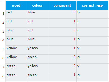
This will create 8 trials, one for each row. Remember how it is the loop components that determine how many times the sequence component repeats. In other words, for every loop around trial_sequence, it will use one of these rows. Our next task is to edit the word component to use these new variables.

Editing the word component¶

If you click on the word component, Green is still in the middle of the screen with green font. We need to click on the settings icon in the top right corner and click on view script. We need to change two things here: the color and text arguments. At the moment, these are static and just present Green every time the component is called. OpenSesame lets you specify arguments using variables defined in a loop by entering the variable name surrounded by square brackets. For color, you should change it to say color = [colour]. This means that every time the component is called, the colour of the word will be determined by the colour variable in block_loop. We can then do the same for word and make sure it says text = [word]. Be very careful with your typing here as the variables are case sensitive. It should be typed exactly as it is in block_loop. One of the biggest causes of experiments not working is typos. You need an eagle eye to spot where you have made a mistake. The script should now look like this:

Click on apply and close in the top right corner and we can move on to keyboard_response.

Editing keyboard_response¶

We can now specify what variable determines a Correct response and enter several Allowed responses. In block_loop, we created a variable called correct_resp to tell OpenSesame what response should be provided. We need to use the same trick as in the script for word and enter ‘[correct_resp]’ to tell OpenSesame it should look for a variable. We then need to specify the four different responses that are allowed (g; r; b; y) in the Allowed responses box. It is important that the letters are separated by a semicolon and not a comma. After this, you should have a window that looks like this:

Test the experiment¶

We can now test it works again using quick run. It should run for 8 trials providing you have followed all the instructions closely. If you get an error message, use the instructions to try and locate the problem. It will probably be a stray typo in one of the variable names you have entered, so make sure it is all typed out exactly as in the instructions.

Increase the number of trials¶

Now that we know everything works fine, we can scale the experiment up to provide more trials. If we go back to block_loop, we can change the Repeat value to 4. This repeats all of our conditions 4 times to produce 32 trials. You will find that cognitive tasks repeat stimuli many times and take the average. We could specify all 32 trials in the block_loop grid, but doing it like this is much more efficient. One of the important settings to highlight now is Order. The default is random, which mixes our 8 rows up every time we run the experiment. This is usually the setting you will use as randomising the order helps to avoid presentation order being a confounding variable. The alternative is sequential. This calls the conditions in the exact order that you wrote them in. This can occasionally be useful if the order of presentation is important.

Run the experiment full screen¶

Now it is time to run the experiment in full screen (the single green arrow) and enter a subject number. In other places, this could be called a participant number or code, but they mean the same thing. It is just the method you are using to label each participant. When you run an experiment, you will need to label all of your participants. OpenSesame asks you to provide a number, and then asks you to specify where you want to save the file. Make sure you create an easily identifiable folder to store your data. When it comes to saving the file, it is better to name your file clearly with a three digit participant number, e.g. stroop-001. This makes it easier to find and organise the file later, and creating a three digit code helps with ordering the files. Click save and run all 32 trials. We will now take a look at the data to see how we could analyse it.

Analysing response time data from the Stroop task¶

Every time you run the experiment, OpenSesame saves the data as a .csv file. This stands for comma-separated values. If you have Microsoft Excel or Openoffice on your computer, you should be able to double click on the file and open it. As we told the logger we want every variable saving, we get many columns. The file should have 32 rows of data and look similar to this:

We do not need every value here, but it is safer to save everything and use what we need. The key variables for analysing the data in this experiment are congruent, correct, and response_time. We can use SPSS to import and process the data for us and see whether we can see the Stroop effect in 32 trials. There are two versions to the import instructions depending on whether you are using version 23 or 25 of SPSS.

Importing the data in SPSS version 23¶

Open SPSS and select open new dataset. This will present you with a blank data view screen to work from. In the main menu, click File > Open > Data. This will present you with a box to Open Data in. In order to open the data file, you will need to change Files of type to CSV (*.csv). If you do not change this, SPSS will just look for SPSS .sav data files. At the top of the box there is a drop-down menu called Look in. This is where you need to search to find where you saved the data on your computer. The window should look like this:

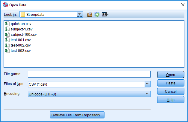
Select the file you need, and click Open. This will open the Text Import Wizard which requires six steps. 1) We do not have a predefined format, so it should say no by default. Click Next. 2) How the variables are arranged should be set to Delimited, the variable names are included at the top of the file, so it should be set to yes, and the decimal symbol should be set to Period. Some international formats use a comma for the decimal symbol, so if you have data in an international format, this would need changing to Comma. Click Next. 3) The first case begins on line number 2, each line represents a case, and we want to import All of the cases. Click Next. 4) The delimiters should be set to Comma and Space by default, and text qualifier set to Double quote. Click Next. 5) This page provides you with the option to change each variable name, but we can change these later if necessary. Click Next. 6) We do not need to save the file format for future use, and we do not need to paste the syntax. Click Finish to complete the process and the data will be available in the data view screen of SPSS. The whole process from above is shown in the following series of screenshots:

Importing the data in SPSS version 25¶

If you have version 25 of SPSS, you can follow the instructions for version 23 and the process works, but in version 25 there is a more streamlined option for importing data. Open SPSS and select new dataset. There is an option to import data if you click file > Import Data > CSV Data and select the experiment file from where you saved it on your computer. You should have a screen that looks similar to this:

You should not have to change any of the default settings apart from if your data is saved in an international format. Some countries use a comma for a decimal symbol. If this is the case, you would need to change Decimal Symbol to comma. If not, you should just need to press OK.

Processing the data¶

Before we do any analysis, it is important to process the data. Conventionally, we remove any incorrect responses as they may be unreliable. In addition, we should ensure that there are no problematic outliers. In the simplest case, there are response times that can be considered too fast or too slow. Anything below 100-200ms is unlikely to be a real response to the stimulus, as there is not enough time for the participant to perceive the stimulus and make a response. Conversely, response times above 1000-2000ms can be considered too slow and the participant may have been distracted. Response times on simple tasks are usually in the range of 400-700ms. A range of values at each end of the threshold have been presented as there is no one solution. It is important to read articles similar to the study you are conducting to see what they have done and justify your own decisions.

For the next step in the outlier removal procedure, some studies will remove response times above and below certain thresholds to ensure the response times are approximately normally distributed. The most common of these is two or three standard deviations above and below the mean (Lachaud and Renaud, 2011). Despite being commonly used, there is good reason not to do this including being biased by the very outliers they are trying to remove (Leys et al., 2013). If you are interested in using a more robust outlier removal method, Leys et al. (2013) present an alternative using the absolute median deviation. As the outlier removal method differs between studies and topic, in this guide we will just focus on removing incorrect responses, and response times below 100ms and above 1000ms. When it comes to designing your own studies, you will need to look more closely at these articles and methods.

Identifying extreme responses¶

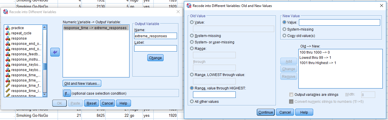
In order to process the data, we will do it in two steps. The first is to create a new variable that defines any outliers beyond 100ms and 1000ms. On the main menu, click on Transform > Recode into Different Variables. Drag response_time into the white box, and type a new Output Variable Name called something like ‘extreme_responses’ and click Change. You should now have a screen that looks like this:

Now click on Old and New Values. This allows us to recode response_time into several values by specifying individual values, or a range of values. Our acceptable response times are 100-1000ms, so we will define three ranges for new values. 1) Click on Range and enter 100 in the first white box and 1000 in the second white box. We then need to specify a New Value for these responses. These are acceptable, so we can code them as 0. Finally click Add, and they will appear in the Old –> New box. Now we want to specify our extreme responses. 2) Click on Range, LOWEST through value and enter 99. This means we are taking the range from the lowest value in response_time to 99, as above 100ms is OK. Select a New Value of 1, and click Add. 3) Click on Range, value through HIGHEST, and specify 1001. Select a New Value of 1, and click Add. You should have a window looking like this:

Click Continue and OK, and SPSS will create a new column called extreme_responses. Any row with a 0 is fine, and any with a 1 is outside of our boundary and considered an extreme response.

Filtering out extreme and incorrect responses¶

We can now get SPSS to ignore any of our incorrect and extreme responses. You can do this in SPSS by clicking on the main menu Data > Select Cases. You then need to select ‘if condition is satisfied’ and click on the ‘if’. We can drag correct into the white box, and make sure it says ‘correct = 1’. This means that we only want cases which has the value 1, indicating a correct response. We also want to exclude our extreme responses, so write ‘& extreme_responses = 0’. This means we only want to include responses within our boundary. It should now say ‘correct = 1 & extreme_responses = 0’. The window should look like this:

Click Continue and then OK, and any responses not meeting our criteria will be crossed out. For my data, there are four cases that are either incorrect or considered extreme. When we run any analyses, this will not be included but does not delete them.

Getting the outcome variable¶

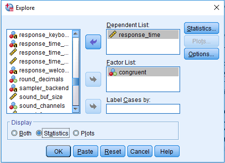
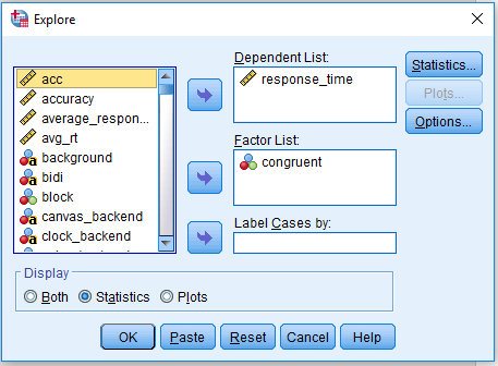
To get the average response for our two conditions, we can click on Analyze > Descriptive Statistics > Explore. Drag response_time into Dependent List and congruent into Factor List. Select Statistics under Display. The window should look like this:

Press OK to produce the output. This will provide the descriptive statistics split by the congruent variable. For the average, we will look at the median response time. Response times tend not to be normally distributed and the mean is often not an appropriate choice. Although it is not perfect, the median is a better choice than the mean in the presence of a skewed distribution with outliers (see Ratcliff, 1993 for a technical paper on dealing with response time outliers). For my data, my median response is 668ms when the colour and word are congruent, and 787ms when they are incongruent. This shows that even in 28 (excluding the four removed) trials you can see the Stroop interference effect. For a real experiment, it would be better to include many more trials as you will get a more accurate estimate, but this is fine for demonstration purposes. If this was entered in SPSS to analyse the data for each participant in an experiment, you would need the variables organised something like this:

participant	congruent_rt	incongruent_rt
1	668	787

Hopefully, you have also seen how it is good to think in advance how you will analyse the data. This last section is one of the most important tips when designing experiments. Design it with the analysis in mind. It is better to realise now that you have overlooked something than when you have already collected data from 20 participants. You will find that you are testing your experiments out several times before the participants in order to catch any mistakes in creating the experiment, and to ensure you have all the variables you need to analyse the data when you have finished.

Tutorial 2. Eriksen Flanker task¶

The Stroop task is probably the most famous task in the whole of psychology. Without knowing the specific details, you might be able to have a go at creating a version of it yourself. However, what would you do if you came across an unfamiliar task that was described in a study you want to extend or replicate?

How do you recreate a psychology experiment?¶

The aim of learning how to use OpenSesame is to enable you to create psychology experiments that you can use in your research. However, what kind of experiments can you create and where do you find out how to create them? In all empirical psychology articles, there will be a method section outlining how the authors conducted their study. If this is written well enough, it should allow you to recreate their study as close as possible. In a lot of studies that use behavioural tasks, the authors provide diagrams of how their tasks are designed. The following diagram is from an EEG study by Rass et al. (2012).

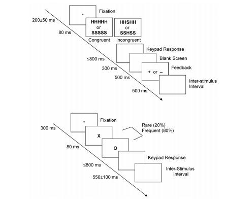
In the second part of this section, we will create the task on the top which is called the Eriksen Flanker task. This follows a similar principle to the Stroop task as it aims to measure the impact of interference on task performance. However, instead of looking at word colour, it uses distracting information. The aim of the task is to identify the middle letter in a five letter string. The four outer letters are distractors, and on some trials they are congruent, and on others they are incongruent. Studies usually find that response times are slower in the incongruent condition than the congruent condition.

What is the structure of each trial?¶

We will go through the diagram above step by step in order to decode how it is designed. In this experiment a trial consists of a central fixation cross which stays on the screen for a random interval between 150-250ms. This randomness is usually introduced to stop participants just mindlessly clicking buttons to predictable stimuli. A stimulus then appears on the screen for 80ms. This period is sometimes called the Stimulus Onset Asynchrony (SOA), or for how long the stimuli remain on the screen. There are two conditions for the stimuli: congruent (HHHHH or SSSSS) or incongruent (SSHSS or HHSHH). For this task, the participant has to identify the middle letter by pressing either the letter ‘s’ or ‘h’ on the keyboard. After the stimulus has disappeared, there is a blank screen where the participant has up to 800ms to provide a response. After the response, a blank screen is presented for 300ms. The participant is then provided feedback to let them know whether they pressed the correct button or not. A ‘+’ is shown for a correct response and a ‘-’ is shown for an incorrect response. Finally, an inter-trial interval (ITI; although confusingly this is called an inter-stimulus interval despite indicating the end of a trial) is shown on the screen for 500ms to indicate the end of a trial.

How is the whole experiment organised?¶

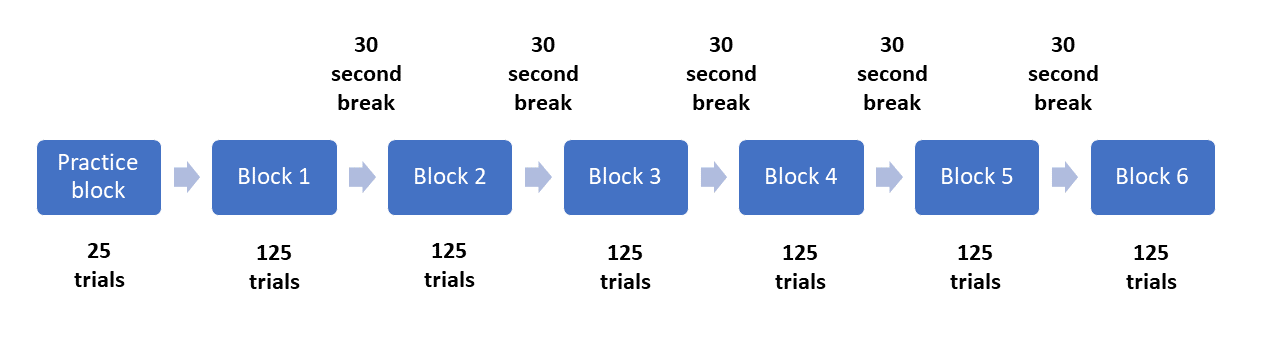
Now that we know how one trial is structured, we can see how many times this is repeated to form a block of trials. In the method section, there are more details about how many trials are included. In order for the participants to understand they are completing the task accurately, they are provided with 20 trials in a practice block. The authors then explain that participants completed four blocks each containing 100 trials for a total of 400 trials. Between each block there is a rest period for the participant, but it does not say how long this period is. We will provide participants with a short 30 second break. Finally, we know that there are an equal number of congruent and incongruent stimuli in each block. As we have two types of congruent and incongruent stimuli, we can take a good guess that each one of these is presented 25 times in each block. The authors provide us with a diagram of each trial, but we can visualise the structure of the whole experiment like this:

This is the amount of information you need from an article to enable you to recreate the task the authors used. This is a particularly good example with the only missing information being the duration of the breaks, a relatively minor detail. You should be prepared to come across substantially less helpful authors that do not provide sufficient details. This is usually the case when it comes to tasks that use images. These are not normally shared or even described. Hopefully this will also demonstrate the importance of fully describing your experiment in a report or dissertation. Try and imagine you are the other researcher trying to recreate the task from your instructions. Now that we know how the task is designed, the next step is to recreate it in OpenSesame.

Creating the Eriksen Flanker Task in OpenSesame¶

For this experiment, we will use the extended template rather than the default. This provides a helpful starting point by creating the basic outline of an experiment. This includes: instructions, a practice block, an experimental block, and an end of experiment message. The template should look like this when you first open it:

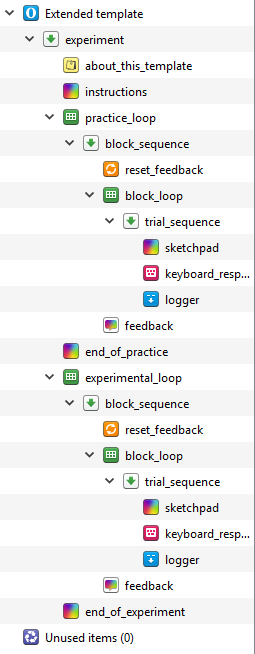
You can permanently delete about_this_template as it just describes the layout of the extended template. You can also permanently delete end_of_practice as we don’t need two messages for this. Start off by changing the name of the experiment by clicking on Extended template in the overview, and changing the name to Eriksen Flanker task by clicking on Extended template in blue. We then want to change the text size to 32, and enter your monitor’s resolution.

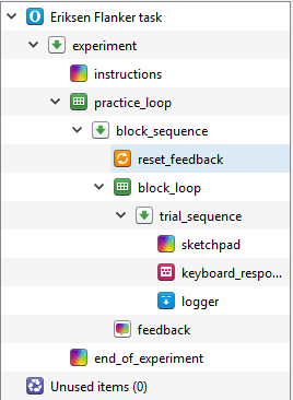
When we made the Stroop task, we only included one block of trials as it was intended to provide a short introduction to creating an experiment using OpenSesame. However, when you create a real experiment, it is a good idea to create a practice block to ensure the participant fully understands what they are doing. One of the helpful features in OpenSesame is the ability to copy and paste a linked component. This means that they are joined, and if you change one of the components, both of them change. This can save a lot of time if the same components are being used with the same settings. In the extended template, the two outer loops (practice_loop and experimental_loop) are independent, but all the components inside them are linked. When you provide people with practice trials, they are usually much shorter than the real experiment as is the case with the design of Rass et al. (2012). Therefore, we are going to delete experimental_loop and edit practice_loop. When we have finished editing practice_loop, we will copy and paste an unlinked version to create another experimental_loop. Right click to delete experimental_loop, and make sure you select permanently delete. If you just click delete, the components will be available in Unused items and it will mess up naming them later. Your Overview should now look like this:

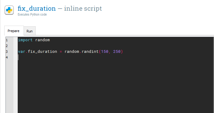
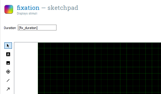
Editing the fixation dot¶

In trial_sequence, there is helpfully a sketchpad component that already includes a fixation dot called sketchpad. Rename this component to fixation. In the trial diagram, fixation is displayed for a random interval between 150ms and 250ms. In the Stroop task, we just set a static duration for 500ms. To create a variable duration, we will need to use our first bit of real Python code. Drag an inline_script component into trial_sequence and place it before fixation. This component allows you to write Python code that can be used in your experiment. Rename it fix_duration as it will control how long our fixation dot is presented for. Within an inline script component, there are two tabs: Prepare and Run. The difference is not important here as we will only be creating a random number. However, if you were to create some complicated stimuli, it can take longer to prepare which affects the timing of the experiment. Therefore, it is better to prepare the stimuli in advance using the Prepare tab, and these can then be presented when necessary using the Run tab. For this example, we will just be writing two lines of code in the Prepare tab. On the first line, type:

import random

It is very important these are all lowercase as Python code is case sensitive. This imports a library called random. A library is a collection of Python code which have specific functions. Random has different functions for creating random numbers. On a new line (it does not matter whether it is on line 2 or 3), we need to create a new variable called fix_duration using the following code:

var.fix_duration = random.randint(150, 250)

This should look like the following:

We will take some time to unpack what this is doing. The first part var.fix_duration is creating a new variable called fix_duration. OpenSesame uses the var object to access and create experimental variables in inline scripts. We use the equals sign to assign fix_duration with a number created by the second part of the code. The second part random.randint(150, 250) is accessing a function within the random library called randint. This creates a random integer (whole number) between two numbers which you specify. As we want a random duration between 150ms and 250ms, we enter 150 and 250. Therefore, at the start of every trial (as we put fix_duration within block_loop), we get a new random value for fix_duration. For example, on the first trial it could be 250, on the second 178, and so on. This discourages the participant from mindlessly responding in a predictable fashion. As we created a new variable, we can use this to determine the Duration of fixation using square brackets. If you type [fix_duration] in the Duration of fixation, you should have a component that looks like this:

Creating a stimulus component¶

Drag a new sketchpad component called stimulus and place it after fixation. Create a text element in the centre of the stimulus screen at coordinates 0,0 and type ‘[stimulus]’. We have not created a stimulus variable in block_loop yet, but we are preempting doing it later. From the trial diagram, we need to change the Duration to 80ms. This displays the stimuli very briefly.

Creating a blank response screen and keyboard response¶

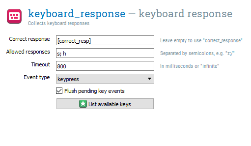
For the participant to provide a response, we need two components. We need a blank sketchpad component which we can call response_screen and place after stimulus. Set the Duration to 0 as we want the time allowed to be controlled by keyboard_response which was helpfully already present from the extended template.

We can edit keyboard_response for this task. In Correct response, we can preempt creating a variable by typing ‘[correct_resp]’. We only need two responses, so type ‘s; h’ in Allowed responses. We want the participant to respond within 800ms, so set Timeout to 800. This means that if the participant takes longer than 800ms to respond, the response is classified as None and incorrect. The keyboard_response component should look like this now:

Creating another blank screen¶

Now we need another blank sketchpad component called blank_screen that has a duration of 300ms. This should be placed after keyboard_response. At this point in the trial, the participant is provided with feedback on whether they pressed the correct button or not.

Creating feedback screens¶

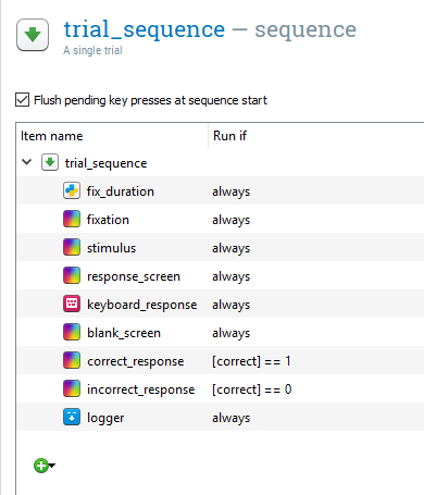
We need two more sketchpad components placed in the centre of both screens called correct_response and incorrect_response placed after blank_screen. Both components should have a Duration of 500ms. We need a text element placed in the centre of both screens. In correct_response, we need a ‘+’ to denote a correct response, and in incorrect_response we need a ‘-’ to denote an incorrect response. If we left the components like this, OpenSesame would display one and then the other. We need to use a bit of Python trickery to control which component is displayed depending on the response. If you click on trial_sequence, you will see a list of all the components within it. There is a second column called Run if. By default, this is set to always, so each component is displayed on every trial. We can modify this and use the correct variable that is updated on every trial. So if the participant pressed the correct button, this would be recorded as a 1, and if they pressed the wrong button, this would be recorded as a 0. Where it says always, change it to [correct] == 1 next to correct_response, and [correct] == 0 next to incorrect_response. The square brackets means we want to access a variable, and 1 and 0 refers to a correct or incorrect response. The two equals signs compares the values either side of the ==. If they match, it is evaluated as true, and if they do not, it is evaluated as false. Therefore, when we have a correct response, correct_response is run, and when we have an incorrect response, incorrect_response is run. At this point, trial_sequence should look like this:

Creating one final blank screen¶

The final component we need here is a final blank screen which Rass et al. (2012) call the inter-stimulus interval. Drag and place a new sketchpad component called isi after incorrect_response and set the Duration to 500ms. The logger component is already in place from the extended template, so we just need to add some variables in block_loop before we can test if the experiment works at this point.

Creating variables in block_loop¶

In block_loop, we need three columns: stimulus, congruent, and correct_resp. These need to be typed exactly as they were in the components from earlier. The stimulus variable should have four rows: HHHHH, HHSHH, SSSSS, and SSHSS. This covers all the stimuli outlined in the trial diagram. The congruent variable should be a 1 if the letters are all the same, and a 0 if the outer letters are different to the middle letter. Finally, correct_resp should be h or s depending on whether the middle letter is a h or s. The block_loop should now look like this:

Time to test the task¶

Now is the time to test out the task using quick run . It should run through all of the components and present four trials. We do not need to modify the instruction components yet as it is only to make sure the trials are presenting as they should do. If you have copied all the instructions exactly, it should work. If you get an error message, try and track down the problem. If it crashes, it will try and provide you with instructions on where the error was. Look for any typos or if you forgot to follow any of the steps.

Editing practice_loop¶

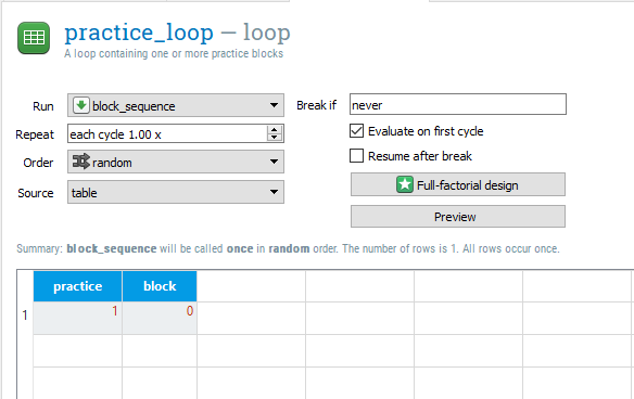
Before we duplicate practice_loop to create a set of experimental trials, we will adapt the loop settings to create some variables for the data file. In practice_loop, there is already one variable and row called practice and yes. We will change this slightly to say 1 instead of yes. Remember we usually use 1 to mean true. Practice trials are not included when you process the data, so this will make it easy to exclude them later on. We will then add a new variable called block with one row and a 0. We are using a 0 as we will be labelling each experimental block as 1-4. The practice_loop component should now look like this:

Creating an experimental loop¶

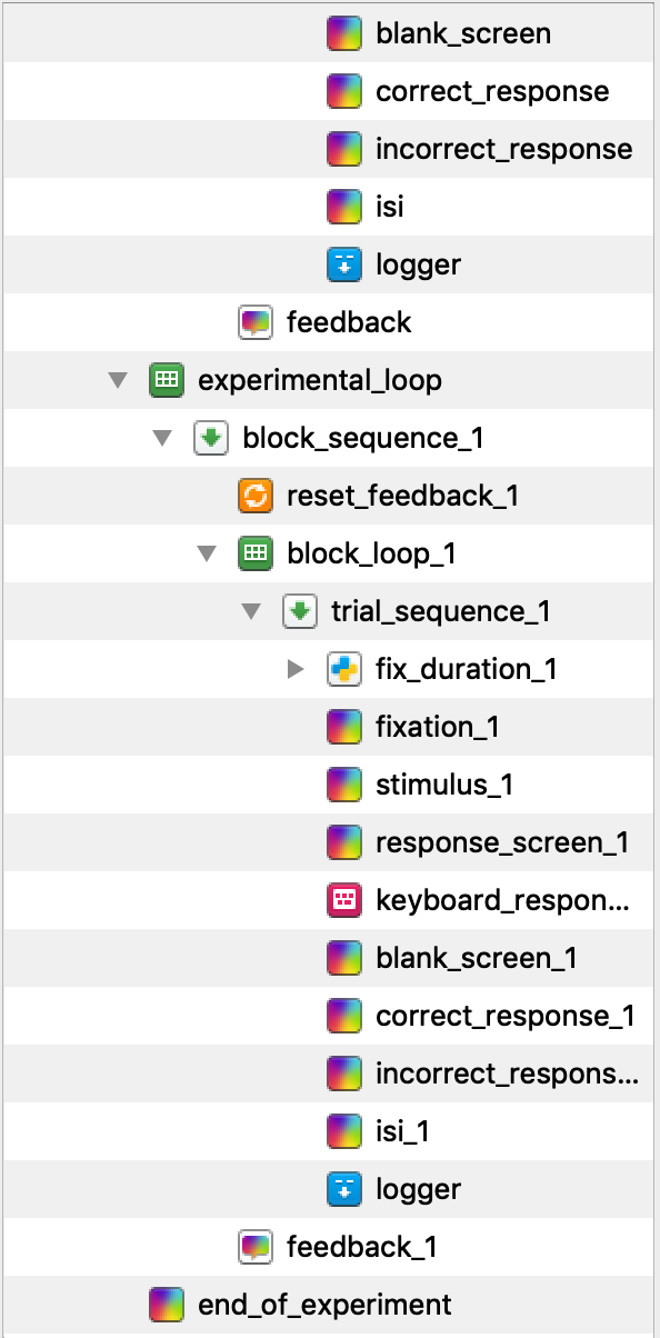
Now is the time to copy and paste practice_loop to create our experimental loop. It is very important that we copy an unlinked version of the component, as we want to add some components without changing practice_loop. As you cannot have duplicate component names, all of the new components will have _1 appended to their names. Change the name of practice_loop_1 to experimental_loop. We also do not want two unlinked logger components. This will effectively cause the data file to be twice as wide as each variable is recorded twice. Permanently delete logger_1 and copy and paste a linked version of logger in its place. You should now have an Overview that looks like this at the bottom (note this is missing some of the components at the top):

Editing experimental_loop¶

We will start by creating some variables in experimental_loop. Instead of block reading 0, we now want four rows with the numbers 1 to 4. This is because we will have four experimental blocks. You can then change the practice variable to have a 0 in each of the four rows as they are no longer practice blocks. Finally, change the Order to sequential so the data file is always organised as blocks 1 to 4. This will come in handy later when we will use the block variable to control when a break screen is displayed. The experimental_loop component should now look like this:

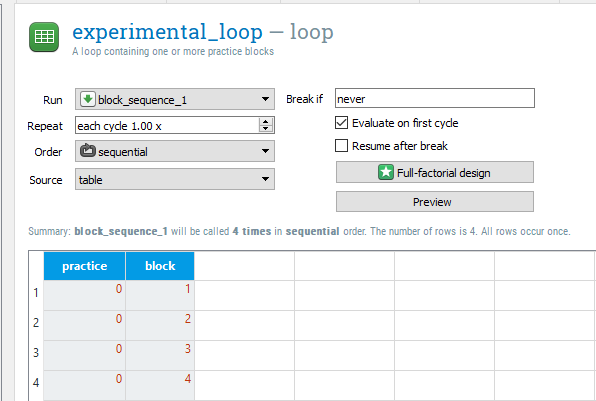
Creating a break for participants¶

After the end of each experimental block, we want to provide the participant with a break. As the final version of the task has 100 trials in each block, it can be mentally draining, so it is a good idea to provide your participants with an opportunity to rest their eyes. We will change feedback_1 to tell them they have 30 seconds to rest. Double click on the existing text when it changes to a grey colour, and write another line to read ‘You now have a 30 second break.’. By default, the font size is 18. Click on the settings icon in the top right corner and click on view script. Change the font size to 32 instead of 18 and click apply and close. We will have to do this for each sketchpad component we edit as changing the default font size only applies to new text elements. Change the Duration to 30000 as this will display the screen for 30 seconds.

Telling the participants when their break is over¶

We then want to create a new sketchpad component called end_break and place it after feedback_1 within block_sequence_1. In this component, we just need a text element informing the participant their break has finished and to press any key to start the next block. Duration is set to keypress by default so you do not have to change this. This is to ensure the participant can begin when they are ready.

Controlling when the breaks are presented¶

If we left it like this, feedback_1 and end_break would run at the end of every block, even at the end of the experiment. This is not necessary, so we can edit the Run if settings in block_sequence_1 to prevent this. Change always to [block] < 4 for both feedback_1 and end_break. This means that these two components will only run on blocks 1 to 3. After the fourth block, we will just get the end of experiment message which tidies the task up. The block_sequence_1 component should now look like this:

Test that the task works again¶

This is the next point where we should make sure the task is working as intended. Use quick run to test it is working with only 4 trials in each block. It is a good idea to keep the number of trials very small at the testing stage, so that if there is a mistake later in the experiment that causes it to crash, you have not spent 10 minutes working through the task. If you followed all the instructions, the task should run and there should only be three breaks.

Increasing the number of trials¶

At this point, the skeleton of the task is complete and working as we want it to. All we have left to do is edit all of the messages to be informative and increase the number of trials. Make sure you edit instructions, feedback, and end_of_experiment. Make sure the participants are informed in feedback they will be starting the main experimental trials when they press a button. We know from the instructions in Rass et al. (2012) that there were 20 practice trials and 100 trials in each experimental block. In block_loop, change the repeat setting to 5 to create 20 trials. In block_loop_1, change the repeat setting to 25 to create 100 trials. You can now run the task full screen to test it out and get a full data set to explore in the next section.

Analysing response time data from the Eriksen Flanker task¶

After running the task, you should have a data set with 420 trials to work with. Follow the same instructions as task one to import the data set into SPSS as a .csv file depending on whether you are using version 23 or 25 of SPSS. Before looking at the reaction times, we will follow the same procedure as task one and remove any extreme and incorrect responses.

Removing unwanted trials¶

Follow the previous instructions from task one to code extreme responses as 1 and acceptable responses as 0. For this experiment, we will also remove the practice trials. If you click on Data > Select Cases, and then if condition is satisfied, we need to specify three criteria: correct = 1 & practice = 0 & extreme_response = 0. Your window should look like this:

If you click Continue and then OK, SPSS will remove the first 20 rows and any incorrect/extreme responses. You will probably notice that you made quite a few errors. The aim of this task in Rass et al. (2012) was to force participants to make several mistakes as they were interested in how participants responded to making errors using EEG. My accuracy was approximately 85% in each block.

Calculating the response time to congruent and incongruent trials¶

We can now look at the difference in respone time between congruent and incongruent trials. In order to calculate the median response time, click Analyze > Descriptive Statistics > Explore. Drag response_time into Dependent List and congruent into Factor List. Select Statistics under Display, and click OK to get the output. The Explore window should look like this:

For my data, my median reaction time to congruent stimuli (congruent = 1) was 330ms, but for incongruent stimuli (congruent = 0) it was 363ms. This shows a small effect of distracting noise on target identification. If you were to run an experiment using this task, you would record these values per participant like this:

participant	congruent_rt	incongruent_rt
1	330	363

Tutorial 3. Go-NoGo task with images¶

For the third task, we are going to create another commonly used cognitive task known as the Go-NoGo task. This measures inhibitory control, or the ability to stop a behaviour once you have started to make it. The standard version of the task presents a series of Go stimuli on the screen, for example a green circle or the letter ‘x’. Every time the participants sees the circle or letter they have to press a button on a keyboard. However, on a small number of trials (20% or fewer), a NoGo stimulus is presented, for example a red circle or the letter ‘o’. This time, they have to avoid pressing the button. Because of how fast the trials progress and the infrequency of the NoGo stimuli, it can be difficult to inhibit the response. The version of the task we are going to recreate is adapted to incorporate different types of images and is based on the task used in Dedandt et al. (2017). This will show you how you can incorporate images into your OpenSesame task.

Recreating the Go-NoGo task¶

Dedandt et al. (2017) were interested in comparing smokers and non-smokers on their ability to inhibit a response. They were also interested if different backgrounds would influence the smokers’ ability to inhibit a response. Therefore, three different backgrounds were used: a smoking cue, a non-smoking cue, and a neutral cue. If we look in the method section of Dedandt et al. (2017), there is a task diagram and a description of the task. We will go through the design of each trial, and how the whole task is structured.

What is the structure of one trial?¶

For the structure of each trial, the authors include this helpful diagram on page 1876 (this is cropped slightly):

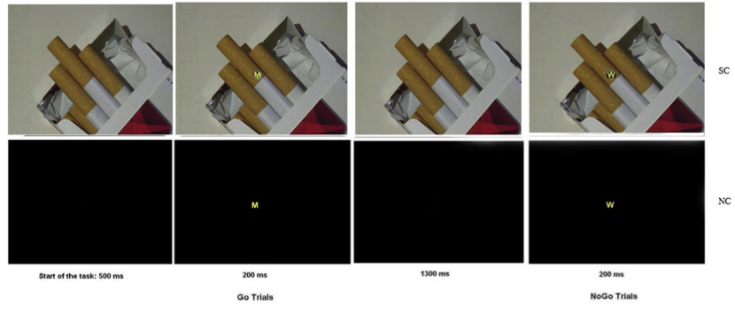
We can see from the diagram that each trial begins with the presentation of the background for 500ms. In contrast to our two previous tasks, there does not appear to be a fixation cross/dot included in this task. A Go or NoGo cue is then presented on the screen for 200ms. On Go trials, this is a letter ‘M’ superimposed onto the background. On NoGo trials, this is the letter ‘W’. After the offset of the cue, there is a 1300ms period where the participant can make a response. The start of the next trial then begins with the next 500ms screen.

What is the structure of the whole experiment?¶

For the structure of the whole task, the study explains there are six experimental blocks. There were five backgrounds used in the task, two smoking images, two non-smoking images, and a blank black background. In contrast to Rass et al. (2012) in the last section, there is quite a bit of missing information that we would need to fully reproduce the task. First, there is no mention of a practice block. Second, the study does not explain that the same black background is used in two blocks. Third, it is not directly explained that one background is shown per block. You can work it out from the introduction and other information in the methods section, but it is not directly specified. These details can be found in another paper which the methodology is based on (Petit et al. 2012). This is a common occurrence, as research teams often produce several publications based on the same method, but to prevent repeating the details in each article, they just reference the first. Finally, it does not explain what kind of break was provided to the participants in between each block. We will give people 30 seconds in order to rest their eyes.

Although we are trying to recreate the task from Dedandt et al. (2017), there is one feature we are going to consciously change: the proportion of Go and NoGo trials. In order to measure inhibitory control, the response to Go stimuli should be be prepotent, meaning you should want to quickly respond, in comparison to the NoGo trials. A long list of studies have been criticised for having too many NoGo trials (Wessel 2017; for a graphical explanation, see FlexibleMeasures). Therefore, Go-NoGo tasks should have a maximum of 20% NoGo trials. As Dedandt et al. (2017) had 30% of the trials as NoGo, we are going to tweak it slightly to be a more valid measure of inhibitory control. Therefore, instead of including 93 Go and 40 NoGo trials per block, we will include 100 Go trials and 25 NoGo trials per block. Similar to the Eriksen Flanker task, we can visualise the structure of the whole experiment like this:

Creating the task in OpenSesame¶

To start this task, we will use the extended template to create the general structure of the experiment. Click on Extended template in the Overview window. Begin by changing the title of the experiment to “Smoking Go-NoGo” by clicking on the blue main title. The resolution will need changing to your monitor’s dimensions, and the default text size should be 32 px. Permanently delete the experimental_loop so we can change the number of trials later without having to change all the blocks.

Adding images to the file pool¶

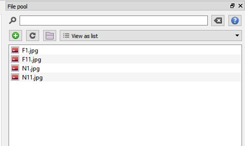
This task will use images (these can be downloaded here) as the background in order to manipulate the type of cues the participant is viewing. If we want to use images in OpenSesame, we need to make them accessible. To do this, we need to add them to the file pool , and click the small green add symbol. This will allow you to browse your computer and select the files. When you have added all four images, the file pool should look like this:

Creating the background screen¶

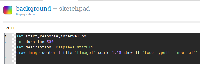
We will create a single trial in trial_sequence using three different components. The first component will be a blank background and we can rename sketchpad to background. The start of each trial is just the background which is presented for 500ms. For each block, the background will be an image we added to the file pool or a plain black screen. This means we need to insert an image element into the centre of the screen at coordinate 0,0. When you click where you want the image, you will be prompted to select an image from the file pool. Select any image as we will be changing it to a variable later.

We need to adapt the script, so click on View script under settings

Creating the response screen¶

The next component we need is to display the cue that participants will need to respond to. To save having to repeat the procedure for the last component, copy and paste an unlinked version of background after the first background, and rename it stimulus_response. This component should have a duration of 200ms. This will be the same screen, but with a response cue and black circle superimposed on the background image. First, select a circle element and make the necessary edits. The image element should look the same as in the previous step. The next element is the circle element. In the figure from Dedandt et al. (2017), we can see the circle is solid black. By default, the color of the circle is set to white and not filled (indicated by fill = 0). Change color to black, and fill to 1. Change the radius (r) to 19 as this just covers the size of the text. Now we need to edit the text element. Change color to yellow to be consistent with the original study, and change the text to [stim_letter]. This is short for stimulus letter and we are preempting another variable we will set in the loop. The script for stimulus_response should now look like this:

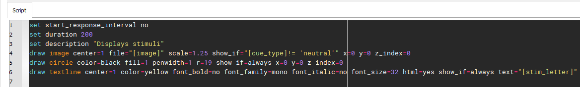
The final thing to note here is the order of the elements is very important. OpenSesame presents them in layers, so the first element is created first, then the second, and so forth. We need to create the image, then the circle, and then the text. If we had a different order, the text or circle would not be visible, which we do not want. Click apply and close, and we will move on to the next component.

Creating a response screen¶

The final sketchpad component we need here is a plain background again, as the stimulus is only presented for 200ms and then disappears. Copy and paste another unlinked version of background after stimulus_response. Change the name to background_response and set the duration to 0. We will be using keyboard_response to control the duration. In keyboard_response, change Correct response to [correct_resp], Allowed responses to ‘m’ as this is the only response we will need, and Timeout to 1300. The logger is already there, so these are all the components we need. We can now start to add in all the variables we have preempted into block_loop.

Defining variables in block_loop¶

There are three variables we need to change on a trial by trial basis. The first variable we want to define is not relevant for the experiment, but it will be helpful for data analysis later. Label the first variable trial_type and enter four rows of ‘go’ and one row of ‘nogo’. In the second column, type stim_letter to control which letter we are presenting. For each ‘go’ trial enter a capital ‘M’, and for the ‘nogo’ trial enter a capital ‘W’. Finally, create a third variable called correct_resp. For each ‘M’ in stim_letter, write a lowercase ‘m’. For the ‘nogo’ trial where we have a ‘W’, write ‘None’. As we are testing the participant’s ability to resist making a response on ‘nogo’ trials, the correct response should be nothing at all. This means we want keyboard_response to time out, which OpenSesame records for the response as ‘None’. Therefore, if we enter ‘None’ for correct_resp, we will get an accurate recording for correct responses and accuracy in the data file. These are all the variables we need to define in this loop component. The loop should look like this when you have finished:

Defining the background image in practice_loop¶

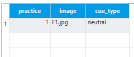
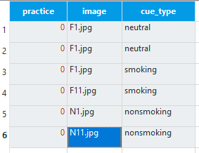
At this point, you may be thinking where we will define the background image. We saw from Dedandt et al. (2017) that we want one image to be presented per block in order to display the same background for a long period of time. Therefore, we are going to define the background image in the outer loop called practice_loop. As this is the practice loop, we only want one block to let the participant try out the task and make sure they understand what they’re doing. The first variable should be practice, and this should be set to 1 to indicate true. The second variable should be ‘image’ and set to ‘F1.jpg’ in reference to one of the images we saved in the file pool. Finally, we need a variable called ‘cue_type’ with one row set to ‘neutral’. During the practice block, it is best to avoid using stimuli that will be in the experimental blocks as the participants may get used to it. We are only defining this image here as we need the image to exist in our file pool or the experiment will crash. However, as we are setting cue_type to ‘neutral’, the image will not display because of how we defined the show_if argument in the image elements. For the practice block, we will just present the participants with a blank black screen. The practice_loop component should now look like this:

Test the experiment¶

At this point, we can test the experiment to make sure it works in its current form. If everything has been defined correctly, you should be able to quick run the experiment and complete five trials. Remember you should avoid making a response when the letter ‘W’ appears.

Creating the experimental_loop¶

Now that we know the task works in principle, we can scale it up to include experimental blocks and change the background image. Copy and paste an unlinked version of practice_loop and place it after end_of_practice. We do not need end_of_practice, so you can permanently delete it. The overview of your experiment should now look like this:

Rename practice_loop_1 to experimental_loop, and permanently delete logger_1. Copy and paste a linked version of logger in the place of logger_1 after keyboard_response_1. This will ensure we have a tidier data file.

Specifying the background images¶

We can now edit experimental_loop to control the background image on each block. The first row should already be there from copying and pasting the loop. This can stay the same as we need one black background screen. All you need to change is practice to 0 as this is now the experimental loop. We will create five more blocks. The image column should have five more rows with F1.jpg, F1.jpg, F11.jpg, N1.jpg, and N11.jpg. For the first two instances of F1.jpg, cue_type should be ‘neutral’ to create two blocks with a black background. For the remaining images starting with ‘F’, cue_type should be ‘smoking’, and for the images starting with ‘N’, cue_type should be ‘nonsmoking’. All the rows should have a 0 for practice. The experimental_loop component should now look like this:

Order should be kept as random, as we want a new order of experimental blocks per participant. At this point, we can test the experiment again using quickrun in order to be certain that all the images are displaying properly and the blocks are presenting as we want them to. One image should be presented in each block, apart from two blocks will just have a black background.

Editing the instruction components¶

Now we can focus on tidying up the instructions. The first thing to change is instructions. Here you can edit the text and explain to prospective participants that they need to press the letter ‘m’ when they see an ‘M’, and withhold a response when they see a ‘W’. Remember for any text you are editing, you will need to change the font size to 32 manually by editing the script. In feedback, we need to explain to the participants that they will begin the experimental trials when they press a button. In feedback_1, we need to explain to the participants that they have a 30 second break. Make sure you change the duration to 30000. We now need to insert a new sketchpad component called end_of_break after feedback_1. Write a message explaining to participants that their break has finished and ensure they can start the next block with a keypress. Finally, change end_of_experiment to thank the participants for their time and they can exit the experiment by pressing any button.

Controlling when the breaks are presented¶

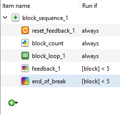
In the last experiment, we stopped feedback_1 and end_of_break from appearing after the final block. Each block was identical, so we just presented each block sequentially and used the number of the fourth block to stop the two components from appearing. However, this time it is not so simple. We cannot simply label each block 1 to 5 as they are being randomly presented. What we need is to label each block as we go along so the background is free to be randomly presented. We can do this by inserting two inline script components called block_count between reset_feedback_1 and block_loop_1 in experimental_loop. Here we need to write var.block = var.block + 1 in the prepare tab. For each loop around experimental_loop this assigns var.block to equal the previous value for block plus one. The positioning of these two inline script components is very important. We want block_start to be outside of experimental_loop as we do not want it to be reset to 0 on on each cycle around the loop. We also want block_count to be in experimental_group and not block_loop_1. If we placed it in block_loop_1, it would increase by one on each trial. We want it to increase by one on each block, so by the time we get to the fifth block, block will equal 5. This means that we can enter some short Python code into block_sequence_1 to control when feedback_1 and end_of_break are run. Where it says always, change it to [block] < 5 for feedback_1 and end_of_break. The block_sequence_1 component should now look like this:

Test the experiment one last time before we increase the number of trials. Use quickrun to test the experiment in a separate screen. The two break screens should not appear after the final break.

Increase the number of trials¶

In block_loop, change the number of repeats to 5 to create a practice block featuring 25 trials. In block_loop_1, we need to set the number of repeats to 25 in order to create 125 trials per experimental block. The experiment should now be in its completed form providing all the instruction components have been edited to be informative to the participants.

Test the experiment full screen¶

You can now run the experiment full screen to get a data set ready to analyse in the next section. At 750 trials, this is a pretty hefty task so it will take approximately 20-30 minutes to complete.

Analysing the data from the task¶

The Go NoGo task provides you with a few options for what you can use as your outcome variable. In the original study by Dedandt et al. (2017), they report three different outcomes: reaction times on Go trials, omission error rates (not pressing a button on Go trials), and commission error rates (pressing a button on Nogo trials). We will go through how you can calculate each one. However, if you were to use this task yourself, it is important to think about which measures you are interested in. Try and avoid analysing several outcomes and seeing which one works unless you are specifically conducting exploratory research.

Import the csv data into SPSS¶

Follow the instructions from the first task for importing the .csv data file from the experiment. You should have a screen that looks like this with 775 rows including the practice trials:

Coding extreme responses¶

This time we do not need to take out the incorrect responses as they are important for calculating the error rates. However, we still need to remove the 25 practice trials and extreme responses. Because of the nogo trials, we need to think more carefully about how we exclude extreme responses. In the previous tasks, we excluded any response outside of 100-1000ms. However, on nogo trials, the participants should not be pressing anything, which means the response time should always be 1300ms. This would mean all nogo trials would be excluded if we performed the same extreme response removal procedure. Click on Transform > Recode into Different Variables. We can still call the Output Variable “extreme_response” and create the same Old and New Values. As a reminder, the menus should look like this:

Click Continue on the Old and New Values screen. In the Recode into Different Variables menu, click on If… above the OK button. Click Include if case satisfies condition and type trial_type = ‘go’. This means we only want to recode go trials, and ignore nogo trials for now. The menu should look like this:

Click Continue and OK, and the extreme_response column should have a 1.00 for extreme go responses, 0 for acceptable, and blank for nogo trials. The blank responses are created as we told SPSS to just recode go responses. Blank entries are not helpful, so we need to fill them in with a 0 for nogo trials.

Click Transform > Recode into Same Variables. This allows us to change values in the same column, rather than computing another one as we have done previously. Drag extreme_response into Numeric Variables and click on Old and New Values. Click System-missing under Old Value and type 0 into Value under New Value and click Add. The screen should look like this:

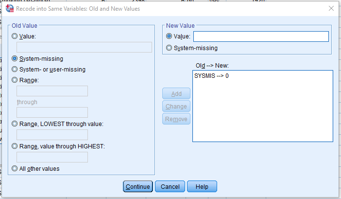If you click Continue and OK, this will fill in all the missing values with a 0 for our nogo trials.

Removing extreme responses and practice trials¶

We can now select cases using this the extreme_response column. Click on Data > Select Cases, and if condition is satisfied. As we labelled the blocks starting as 0, we can select block > 0. This will remove the practice block and leave blocks 1-6. In addition, include extreme_response = 0. The select cases window should look like this:

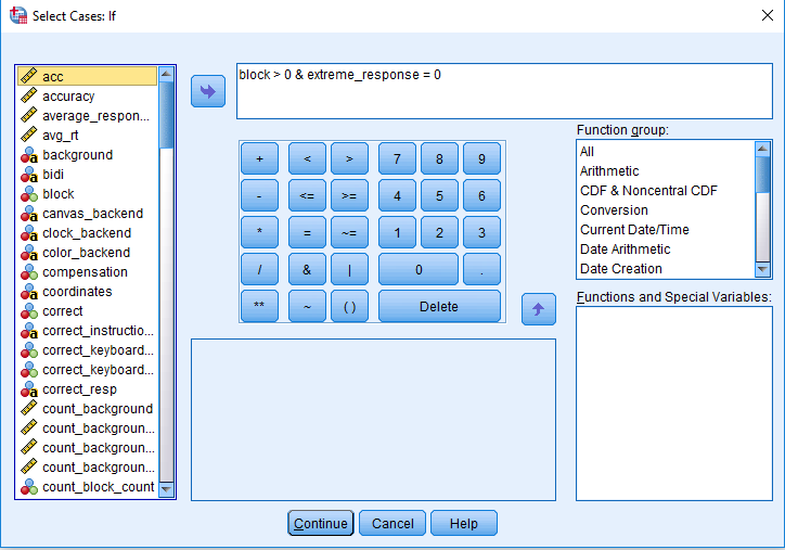Click continue and OK to apply the select cases. This will cross out any practice trials and extreme go responses. Remember we want to retain incorrect responses for the analysis of error rates.

Calculating error rates¶

We can calculate the omission and commission error rates together. Click on Analyze > Descriptive Statistics > Explore. Drag the correct variable In the Dependent List box. One of the benefits of coding correct and incorrect responses as 1 and 0 is calculating the mean provides you with the percentage correct. For example, if you have 100 trials and get 75 correct, the mean of the correct variable would be 0.75 (75%). Now drag cue_type and trial_type into Factor List. Finally, we only need statistics so click Statistics under display. If we pressed OK now, we would get two outputs, one table for correct split by cue_type, and one table for correct split by trial_type. SPSS can be stubborn and does not provide us with the option to split correct by the combination of cue_type and trial_type through the menu. However, we can edit the underlying syntax to get SPSS to do it. Click on Paste and this is the underlying syntax that SPSS uses to specify the analyses. You should have a window that looks like this:

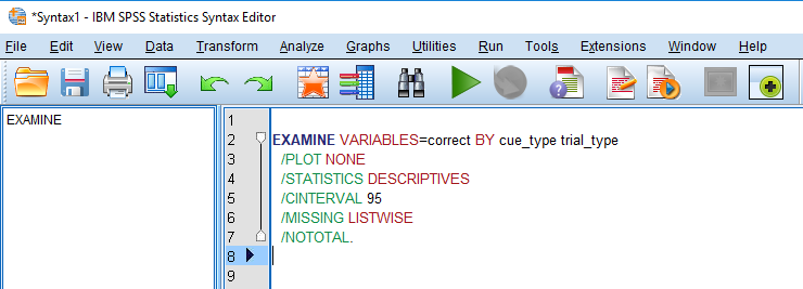We are interested in the first line of syntax. This is telling us we are examining correct by cue_type and trial_type. In order to examine correct by the interaction of the two variables, we simply need to add a star (*) between the two factors. This tells SPSS we want the combination of the two variables. You should now have a syntax screen that looks like this:

In order to get the statistics, we need to click the big green arrow to run the syntax. In the SPSS output, the first table should look like this:

This tells us we should have the information we want and correct is broken down by the combination of cue_type and trial_type. Note there are some missing go trials because of extreme responses. In order to get our first two outcome variables, we need the mean of correct for each combination of the variables in the Descriptives table. The Descriptives table should look like this:

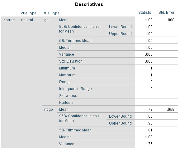
This is a shortened version that shows the output for the neutral cue_type. In order to get the same outcome variable as Dedandt et al. (2017), we need to subtract the mean from 1 for both go and nogo trials. For my data, I would record the different conditions like this in my data file:

Participant	neutral_go	neutral_nogo	smoking_go	smoking_nogo	nonsmoking_go	nonsmoking_nogo
1	0	0.22	0	0.20	0	0.22

This shows that I did not make any omission errors, and my commision error rate was around 20% for each cue condition.

Reporting greater precision¶

SPSS usually reports to two decimal places, which is fine for most purposes, and it is the precision reported in the original article. However, if we wanted a more precise answer, you can see the full number by double clicking on the table and clicking on the cell you are interested in. It should look like this:

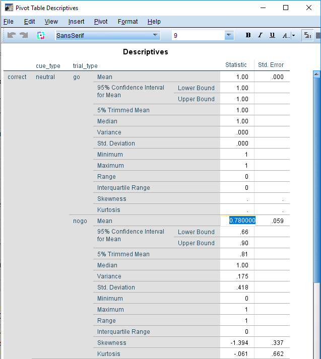
Calculating the response time to go stimuli¶

Calculating the median RT follows the same process as before but using response_time as the dependent variable instead of correct. This time we do have to remove incorrect responses as they may be an unreliable source for the response times. Edit the Select Cases menu and add correct = 1. It should now read: block > 0 & extreme_response = 0 & correct = 1. In order to calculate the median RT, follow the instructions from the last example for the explore menu but replace correct with response_time. When you click paste and add the * between the two factors, the syntax window should now look like this:

All that we replaced is response_time before BY cue_type * trial_type. We could have even wrote this in the syntax ourselves if we typed it exactly as it is in the data file. Press the green arrow to run the syntax again. For the descriptives table in the output, you should have something that looks like this:

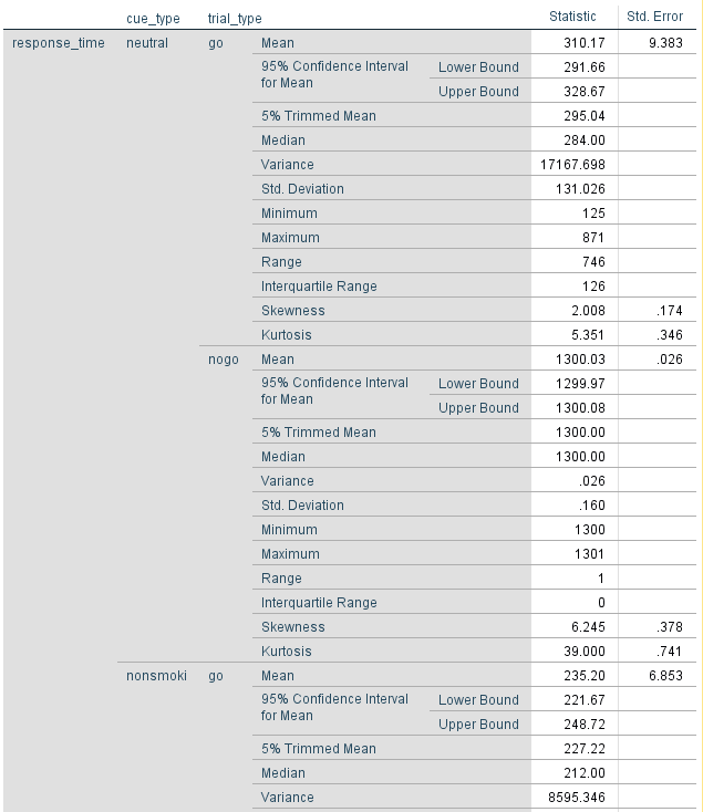
We are only interested in the go trials this time, so we only need to record three values. For my data I would record it like this:

participant	neutral_rt	smoking_rt	non-smoking_rt
1	284	213	212

Tips for Debugging Experiments¶

Debugging an experiment requires problem solving and can be considered a skill in itself. It is similar to the process of science. You have a hypothesis about a problem you are facing. You systematically test the sources of the problem until you isolate it, and then fix the problem. Most of this guide is based on using the OpenSesame GUI, and you will generally encounter fewer bugs than if you were to write your experiment using scripts. However, you will still encounter problems with implementing your ideas. Perhaps your images are not presenting how you want them to, or your feedback is not working. Solving these problems is very similar to solving problems in code. Some of this advice is taken from the excellent book on another Python based experiment builder called PsychoPy (Peirce and MacAskill, 2018).

Steps to take when debugging¶

Read the error messages carefully. If your experiment crashes, OpenSesame does its very best to tell you what caused the problem. Take task three as an example. I run the experiment, and as soon as I press a key after the instructions, the experiment closes and I get the following message:

OpenSesame provides us with a reason for the experiment crashing: thevariable “cuetype” does not exist. At this point, you realise youmissed the underscore and it should be “cue_type”. Not all of theproblems will be this easy, but you should be directed by OpenSesameto the simple fixes.

Look for typos carefully. In my own experience, a stray typo is one of the most common causes of an experiment crashing. As Python is case sensitive, it can be difficult to spot the difference between image and Image. Likewise, the difference between colour and color may be hard to spot. If you are struggling to find typos, you may just be too tired. Make sure you take frequent breaks to prevent being fatigued.
Test your experiments in a separate window. When testing your experiments, always run it in a separate window until you know it works. If you run your experiment full-screen, you may have made a mistake that causes it to freeze and you will be unable to escape it. At best, you just have to restart your computer. At worst, you may have lost an hour’s worth of work if you did not save it beforehand.
Be methodical. If you do not know the source of the problem immediately, change one thing at a time until the experiment works. In an ideal world, get into the habit of testing your experiment after every addition. This means you should know which addition caused the problem in the first place. You can then investigate what it is about that addition that caused the problems.

Asking for help¶

The aim of this guide is to provide you with support to create experiments on your own. However, there will be times where you do not know how to put your idea into practice, or you cannot figure out what is wrong with your experiment. If you are asking for help, the person you are asking will not be very happy if you just say “it doesn’t work”. They will be very grateful if you can break it down and say “I have tried these steps, but it does not work”, or “I have narrowed it down to X, but I cannot work out what is wrong with it”. In my experience, the act of writing down the steps you have taken to solve the problem can often lead you to the solution yourself as you see the bigger picture.

Glossary¶

Argument A value, setting, or piece of information provided by the user in computer programming, normally in a function. This may also be called a parameter.

Block A collection of trials. Blocks group the trials together with a particular theme (e.g. a unique cue is presented or a different response is required in each block). Alternatively, it justs helps to organise the trials and allow the participant to have a break in between.

Boolean operator A system of algebra used to represent logical propositions, and can provide a binary response of either true or false. For example, whether two words are the same which could be true (dog == dog) or false (dog == cat).

Cue A stimulus that elicits or signals a particular behaviour. This has quite a broad definition. In one experiment, it could be a picture of a cigarette to elicit craving in a smoker, and in the next it could be a shape on a screen that requires a particular response.

Debugging The process of finding and removing errors from your experiment or script. It is an exercise in problem solving.

Fixation cross / dot A small cross or dot (e.g. +) in the centre of the screen to attract the participant’s attention at the start of a trial.

Function A section or unit of a programme that performs a specific task. You can consider it to be a procedure or routine.

Graphical User Interface (GUI) An interface that allows users to interact with the programme using icons and visual indicators. For example, being able to select options through a menu by clicking your mouse on the screen.

Integer A whole number (e.g. 1), not a decimal (e.g. 1.3).

Inter-Stimulus Interval (ISI) The amount of time between two or more separate stimuli.

Inter-Trial Interval (ITI) The amount of time between separate trials.

Loop Controls the repetition of several trials and allows things to vary on each repetition.

Python A “high-level general purpose” programming language. See https://www.python.org/ for more details.

Response The action of a participant, e.g. the time it takes to press a button (reaction/response time), when presented with a stimulus.

Script A list of commands/code that is executed by the programme, in this case Python.

Stimulus An object or event that signals a response.

Stimulus Onset Asynchrony (SOA) The amount of time between the onset of one stimulus and the onset of the next stimulus.

Syntax A set of rules that defines the combinations of symbols that are considered to be a correctly structured document in a particular programming language.

Trial Presenting one or more stimuli and recording a response. Typically trials are repeated many times to calculate the average response.

Exercises¶

Excercise 1. Reuse trial sequence in the flanker task¶

Don’t Repeat Yourself (DRY) is a principle of software development. Why? One main reason is that it helps to avoid redunancy in your code. Moreover, if you change information at one place and forget to do it another place this mistake will be very hard to detect and may get unnoticed for any future users too. Let’s improve the experiment you created during the flanker task tutorial by applying this principle.

At the moment we do repeat ourselves by using a copy of the trial_sequence of the practice block in the test block. Moreover, all objects within the trial_sequence_1(except the logger) are copies too! This is not necessary because the trials in the practice block and the test block are identical. So block_loop_1 can simply run the same sequence as block_loop. So, permanently remove trial_sequence_1 and all the copied objects within it. Then, change the block_loop_1 and let it run trial_sequence instead.

Excercise 2. Change the number of trials in the flanker task¶

Brysbaert and Stevens (2018) have suggested that you need at least 1,600 observations per condition to observe RT effects of around 15 ms in a within-subject design. Assume for a moment that the flanker congruency effect is that small (typically it is larger) and you want to run 10 participants in your study. How many observations do you need for each subject and each congruency level? Use the corresponding number to adapt the number of trials presented in the flanker task you just created.

Excercise 3. Stop practice block when performance is sufficient¶

Change the number of trials in the practice phase to 100. Create a script that counts the number of practice trials. Stop the practice block if at least 10 trials have been presented and the accuracy is at least 50%. Abort the experiment if this criterion is still not met after 100 trials. Tip: to debug your script, use lower trial numbers first.

Excercise 4. Calculate average correct reaction time¶

Manually calculate the average reaction time of all correct responses and all incorrect responses. Compare you findings to the default avg_rt calculated by OpenSesame by showing them in the same object (use a feedback item!) at the end of each trial.

Excercise 5. Counterbalancing: Even or odd participant numbers¶

Advanced level! Open the Stroop task you created during the tutorial. Adapt the correct response by using the numeric button 1, 2, 3, and 4 of the keyboard. Use python code to generate the correct response for the four colors. For even-numbered participant numbers (version 1), use the following mapping:

red > 1

green > 2

blue > 3

yellow > 4

For odd-numbered participant numbers (version 2), use the following mapping:

red > 3

green > 4

blue > 1

yellow > 2

Indicate the correct mapping in the instructions.

Note: do not create two versions of the same experiment, just program the counterbalancing in one file. Do not forget to log the version number. Check whether your solution works properly.

When writing the script, try two different methods: 1) using the experimental variable subject_parity (see https://osdoc.cogsci.nl/3.3/manual/variables/) and 2) using the modulus operator % 2 on subject_nr.

References¶

Brysbaert, M., & Stevens, M. (2018). Power analysis and effect size in mixed effects models: A tutorial. Journal of cognition, 1(1).

Detandt, S., Bazan, A., Schröder, E., Olyff, G., Kajosch, H., Verbanck, P., & Campanella, S. (2017). A smoking-related background helps moderate smokers to focus: An event-related potential study using a Go-NoGo task. Clinical Neurophysiology, 128(10), 1872–1885

Mathôt, S., Schreij, D., & Theeuwes, J. (2012). OpenSesame: An open-source, graphical experiment builder for the social sciences. Behavior research methods, 44(2), 314-324

Lachaud, C. M., & Renaud, O. (2011). A tutorial for analyzing human reaction times: How to filter data, manage missing values, and choose a statistical model. Applied Psycholinguistics, 32(2), 389-416.

Leys, C., Ley, C., Klein, O., Bernard, P., & Licata, L. (2013). Detecting outliers: Do not use standard deviation around the mean, use absolute deviation around the median. Journal of Experimental Social Psychology, 49(3), 764–766.

Peirce, J. and MacAskill, M. (2018). Building Experiments in PsychoPy. London: SAGE.

Petit, G., Kornreich, C., Noël, X., Verbanck, P., & Campanella, S. (2012). Alcohol-related context modulates performance of social drinkers in a visual Go/No-Go task: a preliminary assessment of event-related potentials. PloS one, 7(5), e37466

Rass, O., Fridberg, D. J., & O’Donnell, B. F. (2014). Neural correlates of performance monitoring in daily and intermittent smokers. Clinical Neurophysiology, 125(7), 1417–1426

Ratcliff, R. (1993). Methods for Dealing With Reaction Time Outliers. Psychological Bulletin, 114(3), 510–532.

Wessel, J. R. (2018). Prepotent motor activity and inhibitory control demands in different variants of the go/no-go paradigm. Psychophysiology, 55(3), 1–14

Python exercises: Conditionals

Chapter 4 - Functions

Experimentation 1

Stroop, flanker, and go-nogo tasks in OpenSesame

Contents

Stroop, flanker, and go-nogo tasks in OpenSesame¶

Tutorial 1. Stroop Task¶

Creating the Stroop task¶

Creating a new experiment¶

The building blocks of creating an experiment¶

Creating the fixation dot¶

Creating the word component¶

Creating the keyboard response component¶

Creating a blank screen¶

Creating the logger component¶

Creating the end of experiment screen¶

Modifying the welcome message¶

Time to test the experiment¶

Manipulating the presentation of word and colour¶

Editing the block_loop component¶

Editing the word component¶

Editing keyboard_response¶

Test the experiment¶

Increase the number of trials¶

Run the experiment full screen¶

Analysing response time data from the Stroop task¶

Importing the data in SPSS version 23¶

Importing the data in SPSS version 25¶

Processing the data¶

Identifying extreme responses¶

Filtering out extreme and incorrect responses¶

Getting the outcome variable¶

Tutorial 2. Eriksen Flanker task¶

How do you recreate a psychology experiment?¶

What is the structure of each trial?¶

How is the whole experiment organised?¶

Creating the Eriksen Flanker Task in OpenSesame¶

Editing the fixation dot¶

Creating a stimulus component¶

Creating a blank response screen and keyboard response¶

Creating another blank screen¶

Creating feedback screens¶

Creating one final blank screen¶

Creating variables in block_loop¶

Time to test the task¶

Editing practice_loop¶

Creating an experimental loop¶

Editing experimental_loop¶

Creating a break for participants¶

Telling the participants when their break is over¶

Controlling when the breaks are presented¶

Test that the task works again¶

Increasing the number of trials¶

Analysing response time data from the Eriksen Flanker task¶

Removing unwanted trials¶

Calculating the response time to congruent and incongruent trials¶

Tutorial 3. Go-NoGo task with images¶

Recreating the Go-NoGo task¶

What is the structure of one trial?¶

What is the structure of the whole experiment?¶

Creating the task in OpenSesame¶

Adding images to the file pool¶

Creating the background screen¶

Creating the response screen¶

Creating a response screen¶

Defining variables in block_loop¶

Defining the background image in practice_loop¶

Test the experiment¶

Creating the experimental_loop¶

Specifying the background images¶

Editing the instruction components¶

Controlling when the breaks are presented¶

Increase the number of trials¶

Test the experiment full screen¶

Analysing the data from the task¶

Import the csv data into SPSS¶

Coding extreme responses¶

Removing extreme responses and practice trials¶

Calculating error rates¶

Reporting greater precision¶

Calculating the response time to go stimuli¶

Tips for Debugging Experiments¶