Wrangling behavorial data generated by OpenSesame¶

Introduction¶

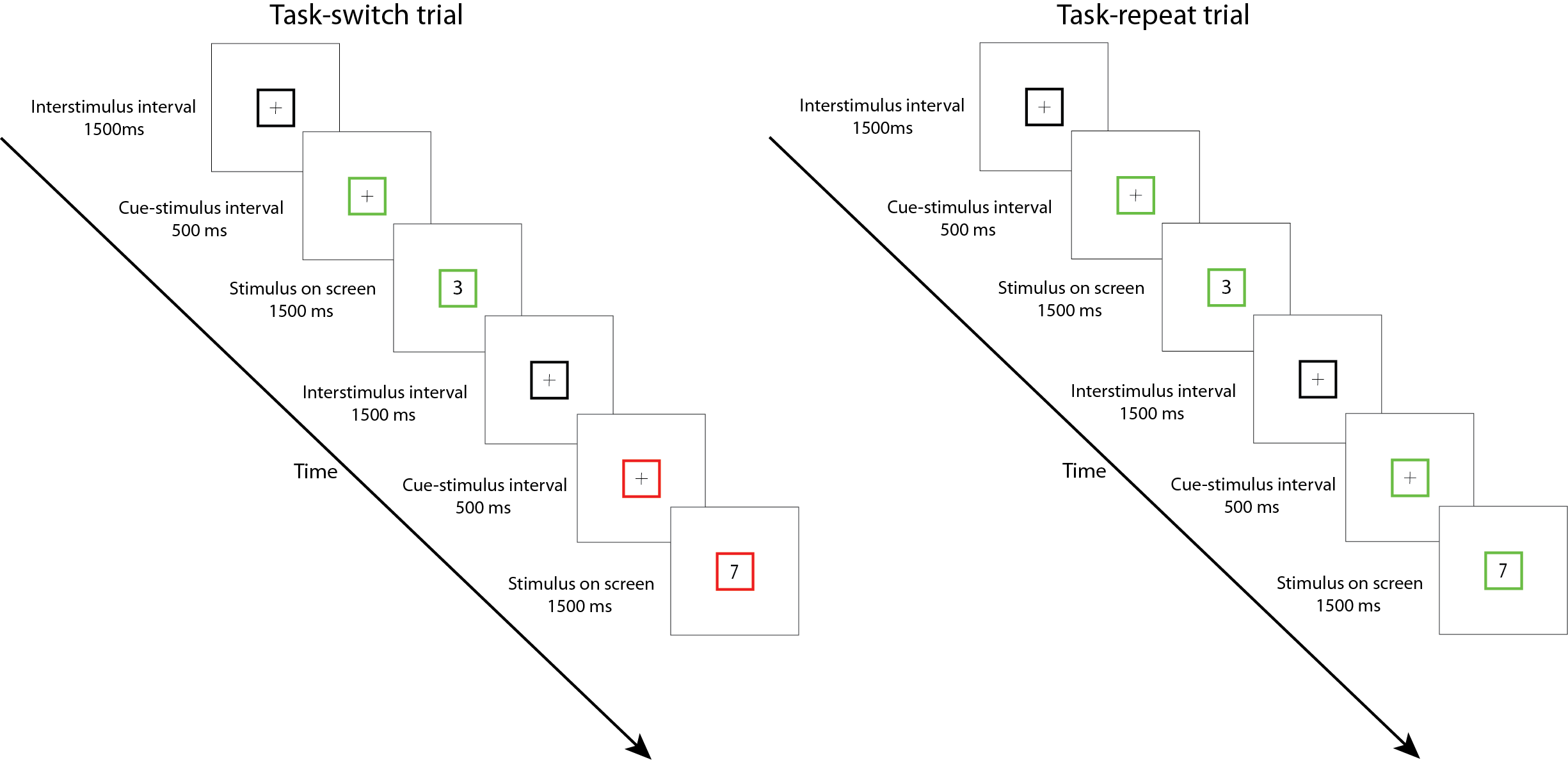
You build the experiment and ran your first two participants. Now, it is time to take a look at the data you have collected. We will be working with a dataset of a task-switching study. In this study, the participants had to conduct two tasks separately: they either had to specify with the left or right button whether the number on screen was odd or even (parity task) or they had to specify with the left or right button whether the number was smaller or larger than 5 (magnitude task). The catch is that they were only told which task they had to do 500 milliseconds before the number came on screen on which they had to respond. If they had to repeat the task from the previous trial, we call that a repeat trial. If they had to switch to another task relative to the previous trial, we call that a switch trial. See below for a schematic overview of the experiment:

image info

Each participant goes through two sessions. In one session, they have to switch tasks 75% of the time (high-switch condition). In the other session, they have to switch tasks 25% of the time (low-switch condition). This setup allows us to examine what happens when people have to switch tasks: are they faster or slower? And what happens with their response time when they have to switch tasks a lot? Or very little? Let’s find out.

OpenSesame outputs a comma-separated values (csv) file. This is a very widely used format, and you can painlessly import this file type in Python using the datafile package pandas (as we’ve seen in the exercises and lessons). Let’s import a datafile from two participants and merge those in one file:

import pandas as pd
import numpy as np

# disable chained assignments, you can ignore this line of code
pd.options.mode.chained_assignment = None

# define all the subjects to load in
subjects = [3, 4]

# make an empty list where we store each URL
url_list = []

# loop over every raw file URL and store that URL in the url_list list
for i in subjects:
    url = 'https://raw.githubusercontent.com/JeshuaT/Experimentation1/main/content/10_dataframes/data/subject-' + str(i) + '.csv'
    url_list.append(url)

# read the csv files from the URLs and append in a pandas dataframe
df = pd.concat((pd.read_csv(url) for url in url_list), ignore_index=True)

That’s a lot of columns. In your “logger” file in OpenSesame, the recommended thing to do is to check the box of “Log all variables”. This is the safest option, because it’s easy to remove columns and you would rather not have that you missed an essential variable after doing your experiment. Let’s pick the columns that we need:

# make a list of column names that we want to include
include_columns = ['subject_nr', 'block', 'session', 'congruency_transition_type', 'congruency_type',
                   'correct', 'response_time', 'task_transition_type', 'task_type', 'response']

# make a new df, called df_trim, that only included the columns that are in the "include_columns" list
df_trim = df[include_columns]

# it's always good practice to check the head and/or tail of a dataframe after making/changing it
print(df_trim.head(5))

   subject_nr  block    session congruency_transition_type congruency_type  \
         3      1  lowswitch                        NaN     incongruent   
         3      1  lowswitch          congruency-switch       congruent   
         3      1  lowswitch      congruency-repetition       congruent   
         3      1  lowswitch          congruency-switch     incongruent   
         3      1  lowswitch      congruency-repetition     incongruent   

   correct  response_time task_transition_type  task_type response  
      0      1482.9738                  NaN     parity     None  
      1       706.7057          task-switch  magnitude        a  
      1       855.6105          task-switch     parity        a  
      1       867.8947      task-repetition     parity        a  
      1      1078.9412          task-switch  magnitude        a  

Before we make any changes to the dataframe, we must first be sure that all the columns are in the right type. If we print the data types of each column, we can see that subject_nr is an integer. However, we don’t intend for the dataframe to interpret “3” and “4” as numbers, since it’s simply a categorization. Let’s change that:

print("Column types BEFORE changing: \n", df_trim.dtypes, "\n")

df_trim['subject_nr'] = df_trim['subject_nr'].astype('category')
df_trim['correct'] = df_trim['correct'].astype('category')

print("Column types AFTER changing: \n",df_trim.dtypes)

Column types BEFORE changing: 
 subject_nr                    category
block                            int64
session                         object
congruency_transition_type      object
congruency_type                 object
correct                       category
response_time                  float64
task_transition_type            object
task_type                       object
response                        object
dtype: object 

Column types AFTER changing: 
 subject_nr                    category
block                            int64
session                         object
congruency_transition_type      object
congruency_type                 object
correct                       category
response_time                  float64
task_transition_type            object
task_type                       object
response                        object
dtype: object

Furthermore, the response times are now rounded in the ten-thousandths (four decimal places) of milliseconds. That gives false confidence in our accuracy with measuring response times, which is more in the range of whole milliseconds. Let’s change that using the pandas round function:

# round the response time column and replace the unrounded column values with the rounded column values
df_trim['response_time'] = df_trim['response_time'].round()

# change type of the column to "int" instead of "float". "int" is for whole numbers, "float" is for numbers with decimals.
df_trim['response_time'] = df_trim['response_time'].astype(int)

# check if it worked
df_trim['response_time']

    1483
     707
     856
     868
    1079
       ... 
   699
   583
   731
   438
  1006
Name: response_time, Length: 952, dtype: int32

Alright, it’s getting a bit more uncluttered now. The task-design is so that the last two blocks are different kind of blocks. We don’t have to go in details now, but for further analysis we will have to create a dataframe without block 11 and 12. There are many ways to conditional selection of rows, but here we opt to use the information that we need all blocks with a value smaller than 11.

# Here the last blocks should be 12, lets check by printing the last 5 rows of the block column using the tail function
print("The last block here is 12: \n", df_trim["block"].tail(5), "\n")

# Conditionally select rows based on if the value in the "block" column is lower than 11
df_trim_blocks = df_trim[df_trim['block'] < 11]

# Check to see if the last block is now 10 instead of 12
print("Here the last block should be 10: \n", df_trim_blocks["block"].tail(5))

The last block here is 12: 
  12
  12
  12
  12
  12
Name: block, dtype: int64 

Here the last block should be 10: 
  10
  10
  10
  10
  10
Name: block, dtype: int64

Lastly, it’s a bit confusing that we have only two subjects, but they are called number 3 and 4, instead of 1 and 2. Let’s fix that by replacing subject 3 with subject 1, and subject 4 with subject 2. We can use the replace function of Pandas to achieve this. Then, with the pandas unique function we can verify that the subject numbers have been changed.

# Replace 3 with 1 in subject_nr column
df_trim_blocks['subject_nr'] = df_trim_blocks['subject_nr'].replace(3, 1)

# Replace 4 with 2 in subject_nr column
df_trim_blocks['subject_nr'] = df_trim_blocks['subject_nr'].replace(4, 2)

# Print out all unique values in subject_nr column, should be 1 and 2
df_trim_blocks['subject_nr'].unique()

[1, 2]
Categories (2, int64): [1, 2]

Let’s see what kind of data we are dealing with. The “session” column tells us whether the trial was in the “lowswitch” or “highswitch” condition. This means that we should see less task-switch trials in the “lowswitch” than in the “highswitch” condition. To check this, we can use the pivot table function from pandas. Let’s check:

Note: We will be using the pandas pivot table for most of tutorial. Be aware however that all of this could also be accomplished with the pandas groupby function. Take a look here for more information on the pivot table and the difference between pivot table and groupby

piv_task_transition_exp = df_trim_blocks.pivot_table(
    index=['session'], # Index on session
    columns='task_transition_type', # Group on 'task_transition_type'
    aggfunc='size') # Function to aggregate columns on, here we specify "size"

# Print out the pivot table
piv_task_transition_exp

task_transition_type	task-repetition	task-switch
session
highswitch	82	248
lowswitch	245	85

Hmmm…doesn’t balance exactly but it’s close. It is always good practice to check if the trials count is what you expected. This experiment had a quite complex counterbalancing structure, since the researchers had to counterbalance:

Amount of congruent/incongruent trials
Amount of parity/magnitude trials
Amount of congruent-switch/congruent-repetition trials

All whilst keeping the task-repetition/task-switch rate to 25/75 or 75/25 (depending on the session). Thereby also keeping into account that the first trial of each block does not count as either repetition or switch trial. In complex structures like this, sometimes you cannot aim for perfect counterbalancing, but you can aim for “as good as possible” (hence the slight discrepancy in the pivot table above). Let’s see if we can use a bit more complex pivot table to get a clearer picture if all of this worked out

piv_cong = df_trim_blocks.pivot_table(
    index=['subject_nr'],
    columns=['congruency_type'],
    aggfunc='size') # Function to aggregate columns on, here we specify "size"

piv_cong_transition = df_trim_blocks.pivot_table(
    index=['subject_nr'],
    columns=['congruency_transition_type'],
    aggfunc='size') # Function to aggregate columns on, here we specify "size"

piv_task = df_trim_blocks.pivot_table(
    index=['subject_nr'],
    columns=['task_type'],
    aggfunc='size') # Function to aggregate columns on, here we specify "size"

piv_task_transition = df_trim_blocks.pivot_table(
    index=['subject_nr'],
    columns='task_transition_type',
    aggfunc='size') # Function to aggregate columns on, here we specify "size"

# Add all dataframes to a list
dfs = [piv_cong, piv_cong_transition, piv_task, piv_task_transition]

# Merge the dataframes, axis=1 defines that the new dataframes should be added as columns instead of new rows
pd.concat(dfs, axis=1)

	congruent	incongruent	congruency-repetition	congruency-switch	magnitude	parity	task-repetition	task-switch
subject_nr
1	167	173	166	164	172	168	245	85
2	172	168	163	167	168	172	82	248

We are repeating quite a lot of code. Whenever you notice that happen, you can probably shorten the code. Let’s try it out:

# Specify the columns we want to check
columns_to_check = ['task_type', 'congruency_type',
                    'task_transition_type', 'congruency_transition_type']

# Make an empty list so we can populate this later
dfs = []

# Loop over columns_to_check and make a new pivot table for each column
for column in columns_to_check: # Loops over "columns_to_check"
    piv = df_trim_blocks.pivot_table(
        index=['subject_nr'],
        columns=[column], # The for-loop inserts a new column here on every iteration
        aggfunc='size') # Function to aggregate columns on, here we specify "size"

    # Append the pivot table to our "dfs" list (which was empty initially)
    dfs.append(piv)

# Merge the dataframes that are in the "dfs" list
pd.concat(dfs, axis=1)

	magnitude	parity	congruent	incongruent	task-repetition	task-switch	congruency-repetition	congruency-switch
subject_nr
1	172	168	167	173	245	85	166	164
2	168	172	172	168	82	248	163	167

Nice. It’s cleaner and also way easier to change this code if you want to check another column for example. The counterbalancing looks good enough.

Now we’ll do some first checks on whether the results are what we expect. Let’s first remove all the incorrect trials, we aren’t interested in those at the moment.

df_correct = df_trim_blocks[df_trim_blocks['correct'] == 1]
df_correct

	subject_nr	block	session	congruency_transition_type	congruency_type	correct	response_time	task_transition_type	task_type	response
1	1	1	lowswitch	congruency-switch	congruent	1	707	task-switch	magnitude	a
2	1	1	lowswitch	congruency-repetition	congruent	1	856	task-switch	parity	a
3	1	1	lowswitch	congruency-switch	incongruent	1	868	task-repetition	parity	a
4	1	1	lowswitch	congruency-repetition	incongruent	1	1079	task-switch	magnitude	a
5	1	1	lowswitch	congruency-repetition	incongruent	1	819	task-repetition	magnitude	a
...	...	...	...	...	...	...	...	...	...	...
810	2	10	highswitch	congruency-repetition	congruent	1	321	task-switch	parity	num_6
811	2	10	highswitch	congruency-switch	incongruent	1	844	task-switch	magnitude	a
812	2	10	highswitch	congruency-repetition	incongruent	1	675	task-switch	parity	num_6
814	2	10	highswitch	congruency-switch	congruent	1	1354	task-switch	magnitude	a
815	2	10	highswitch	congruency-repetition	congruent	1	506	task-switch	parity	a

599 rows × 10 columns

We expect people to be slower when they have to switch from task, in comparison to when they can do the same task as on the previous trial. This is what we call switch cost. To show this in a table-format, we can again use the pivot_table function from pandas.

# Check switch costs
switch_table = pd.pivot_table(
    df_correct,
    values="response_time", # The value that will be summarized
    index=["subject_nr"], # The rows to summarize over
    columns=["task_transition_type"], # The columns to summarize over
    aggfunc=np.mean, # Calculate the mean response time per subject per task type
)

# Print out the pivot table, and change it to "int" so we only have whole numbers
switch_table.astype(int)

task_transition_type	task-repetition	task-switch
subject_nr
1	750	888
2	638	675

It is pretty clear that task-switch trials are slower than task-repeat trials, but we can make it even clearer by showing the difference between the two columns. We can make a new column, and input in that column the difference between the task-switch trials and task-repeat trials:

# Do some arithmetics: subtract task-repetition from the task-switch column
switch_table['switch cost'] = switch_table['task-switch'] - switch_table['task-repetition']

# Print out as int to get whole numbers
switch_table.astype(int)

task_transition_type	task-repetition	task-switch	switch cost
subject_nr
1	750	888	138
2	638	675	37

Lastly, you can use the handy function describe to get a quick peek at the response times.

# Use the "describe" function on the "response_time" column, and change the output to "int"
df_correct['response_time'].describe().astype(int)

count     599
mean      725
std       233
min       124
25%       550
50%       656
75%       876
max      1444
Name: response_time, dtype: int32

What we’ve done here is just a subset of the myriad of possibilities how you can change your dataframe in a way that is tidy and gives you a better overview of what you’re dealing with. This cheat sheet gives a nice overview of the things we discussed and more! Use the cheat sheet for the following exercises.

Note: The developers of OpenSesame have also created a Python package for working with column-based and continuous data, called DataMatrix. It’s similar to the Pandas package we’ve been working with in this tutorial, but has some crucial differences in syntax. We have opted for the more versatile and widely used Pandas package, but be aware that the OpenSesame website and tutorials can sometimes refer to DataMatrixes instead of DataFrames.

Lastly, it’s important to know how to save your cleaned dataframe ofcourse! Here we save it as a csv file, using the pandas to_csv function:

df_trim_blocks.to_csv('../11_plotting/data/df_cleaned.csv', index=False)

Experimentation 1

Wrangling behavorial data generated by OpenSesame

Contents

Wrangling behavorial data generated by OpenSesame¶

Introduction¶

Exercises¶

Exercise 1. Correct versus incorrect trials¶

Exercise 2. Remove rows based on two conditions¶

Exercise 3. Outlier removal methods¶

Exercise 4. Implementing the outlier removal methods¶